 Image: Filori, CC BY-SA 4.0
Correlation is not causation, and what is
Across 17 European countries, the number of breeding pairs of white storks correlates with the number of human births, with a correlation coefficient of 0.62 and a p-value of 0.008. Robert Matthews published this in 2000 in the journal Teaching Statistics, to give teachers a clean example, and the explanation is not hard: large countries have more storks and more babies. Country size is a third variable that drives both, and the storks and the births have nothing to do with each other.
Everyone knows the slogan that correlation is not causation. Fewer people can say what a correlation that is not a causation looks like from the inside, and fewer still can say what is a causation. This article does both.
Three ways a correlation lies
The first is the stork case: a confounder, a third variable that influences both. Children with bigger feet read better, because older children have bigger feet and read better. People who drink coffee have more heart attacks, in old studies, because coffee drinkers smoked more. Countries that eat more chocolate have more Nobel laureates, because rich countries do both. In each case the correlation is real and the causal reading is wrong, and the test is to ask whether the relationship survives when the third variable is held fixed. Among children of the same age, foot size predicts nothing.
The second is time. Two quantities that both rise over the years are correlated whether or not they have anything to do with each other, because the years are a confounder. Tyler Vigen's collection of spurious correlations, built by searching thousands of time series for pairs that match, has the number of films Nicolas Cage appeared in against drownings in swimming pools, with a correlation of 0.67, and dozens of pairs above 0.9. None means anything, and that is the point of the collection: with enough series to search, a high correlation between two of them is a certainty.
The third is reverse causation. Towns with more police have more crime; hospitals have more deaths than hotels. The arrow runs from the second variable to the first.
Simpson's paradox and the kidney stones
A confounder can do worse than create a false correlation. It can reverse a true one. In 1986 a study in the British Medical Journal compared two treatments for kidney stones, open surgery and a newer method that removes the stone through a small puncture, in 700 patients. The newer method succeeded in 83 per cent of cases, open surgery in 78 per cent. The newer method looks better.
Split the patients by the size of the stone and the picture reverses. For small stones, open surgery succeeded in 93 per cent (81 of 87) against 87 per cent (234 of 270) for the puncture method. For large stones, open surgery succeeded in 73 per cent (192 of 263) against 69 per cent (55 of 80). Open surgery is better for small stones and better for large stones and worse overall. The original paper by Charig and colleagues is free to read.
The resolution is in the numbers in brackets. Surgeons sent the hard cases, the large stones, to open surgery and the easy cases to the new method. Open surgery's overall rate is dragged down by having treated mostly large stones, and the puncture method's rate is lifted by having treated mostly small ones. Stone size is a confounder that influenced both the choice of treatment and the outcome, and when it is held fixed the comparison changes sign. This is Simpson's paradox, named after Edward Simpson's paper of 1951, and it is a paradox only until you ask who got which treatment.
What establishes a cause
A correlation is evidence of a cause when the two groups being compared differ in the suspected cause and in nothing else that matters. There are three ways to arrange that.
The first and strongest is to assign the cause at random. If a coin decides which patient gets which treatment, then stone size, age, wealth, and every other variable, known and unknown, are on average the same in both groups, and a difference in outcomes can only be the treatment or chance, and the size of chance can be calculated. Ronald Fisher built the theory of randomized experiments in the 1920s for agricultural plots; the first randomized clinical trial, of streptomycin for tuberculosis, was run by Austin Bradford Hill in 1948. Every drug approved since then has passed through this design.
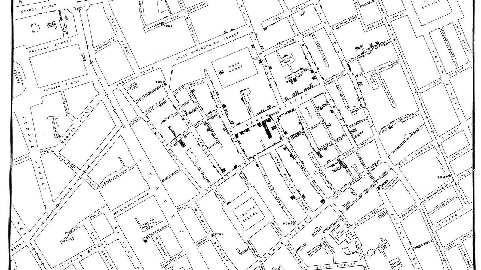
The second is to find a situation where something else did the random assignment. John Snow's two water companies, whose pipes ran down the same streets, assigned households to clean or contaminated water without regard to anything about the households, and the 315 against 37 deaths per 10,000 houses were as good as an experiment. The Vietnam draft lottery assigned young men to military service by birth date, and Joshua Angrist used it in 1990 to measure what service did to their later earnings. These are natural experiments, and the Nobel Memorial Prize in Economic Sciences 2021 went to Angrist, Guido Imbens, and David Card for making them a method.
The third is the hard road of observational evidence, where neither you nor nature randomized. Here the confounders must be measured and adjusted for, as the kidney stone study did by splitting on stone size, and the worry is always the confounder you did not measure. Richard Doll and Bradford Hill could not randomize people to smoke, and their study of 40,000 British doctors from 1951 established the link to lung cancer through sheer weight of evidence: a large effect, a dose-response relation, consistency across many studies, a plausible mechanism, and the fall in risk after quitting. Bradford Hill set out these considerations in 1965, and they remain the checklist for a causal claim without an experiment.
The habit to build
When you meet a correlation, ask three questions in order. What third variable could drive both? Could the arrow run the other way? And how were the two groups formed, by a coin, by an accident, or by someone's choice? The answers decide whether the correlation is a finding or a coincidence, and no amount of statistical significance substitutes for them. The storks had a p-value of 0.008.
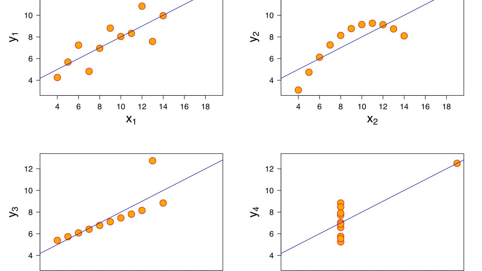
Unit 8 of the Statistics Masterclass works through Anscombe's quartet, the storks, the kidney stones, and the two water companies in that order, and its research spotlight presents Angrist's draft lottery study as the modern form of Snow's comparison. For readers who want the methods themselves, instrumental variables and the potential outcomes framework, the unit's reading list points the way.