 Image: Schutz and Avenue, CC BY-SA 3.0
Same statistics, different pictures
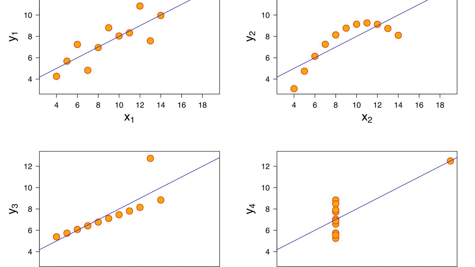
Four datasets, eleven points each. In every one of them the \(x\) values have mean 9 and variance 11, the \(y\) values have mean 7.50 and variance 4.12, the correlation between \(x\) and \(y\) is 0.816, and the least-squares line is \(y = 3.00 + 0.500x\). A statistician given the four tables and no plots would write the same report four times. Plotted, the first is a cloud of points around a line, the second is a smooth curve, the third is a perfect line with one point far off it, and the fourth is ten points stacked at the same \(x\) with one point far to the right holding up the whole regression.
Frank Anscombe, a statistician at Yale University, built the four in 1973 and published them in a short paper in The American Statistician called Graphs in Statistical Analysis. The quartet, as it came to be called, has been in textbooks ever since, and it is the shortest argument there is for a rule that statisticians state and students ignore: plot the data before you compute anything.
The four pictures
The first dataset is what the summary statistics suggest: a linear relationship with scatter. The line fits, the correlation describes the fit, and nothing is wrong.
The second is a parabola. The points lie exactly on a curve that rises and then falls, with no scatter at all. A straight line through it has the same slope and the same correlation as the first dataset, and it is the wrong model. The residuals, the vertical distances from the line, are negative at both ends and positive in the middle, which is the signature of a curve fitted by a line, and a plot of the residuals shows it as clearly as a plot of the data.
The third is a perfect straight line, with a different slope from the fitted one, plus one point that sits far above it. That single outlier pulls the least-squares line towards itself and away from the ten points that lie exactly on another line. Remove it and the correlation becomes 1.
The fourth is the strangest. Ten of the eleven points have the same \(x\) value, 8, and various \(y\) values; the eleventh is at \(x = 19\). With ten points at one \(x\) there is no relationship between \(x\) and \(y\) at all. The entire slope, the entire correlation of 0.816, is produced by the one point on the right. In regression language that point has very high leverage: the fitted line must pass close to it whatever the other ten do. Move it up or down and the slope swings with it.
What Anscombe was arguing against
In 1973 computers had made it easy to calculate regression coefficients and correlations and still awkward to draw a graph, and Anscombe's paper opens by complaining that textbooks and statistical packages treated calculations as the real work and graphs as decoration. He wanted to show that the numbers can be identical when the data are not, and that every one of the four datasets other than the first has something in it that the summary hides: a wrong model, a bad point, a point doing all the work. The graph finds these in a second. The numbers never do.
He was writing in the same decade as John Tukey, whose book Exploratory Data Analysis of 1977 made the case for looking at data before modelling it and gave the field the box plot and the stem-and-leaf display. Both men were arguing that the first thing to do with a dataset is to look at it, and that a statistician who computes a correlation without a scatter plot is driving with the windscreen painted over.
The dinosaur
In 2016 the data journalist Alberto Cairo drew a dataset by hand, 142 points that form a dinosaur, and challenged people to describe it with summary statistics; its mean, standard deviations, and correlation are unremarkable. The following year Justin Matejka and George Fitzmaurice of Autodesk Research took the dinosaur and, by a procedure of moving points a tiny distance at a time while keeping the summary statistics fixed to two decimal places, turned it into twelve other shapes: a star, a circle, parallel lines, an X, a set of dots arranged in a grid. Every one has mean \(x\) of 54.26, mean \(y\) of 47.83, standard deviations of 16.76 and 26.93, and a correlation of minus 0.06. They called the collection the Datasaurus Dozen, and their paper and the data are free.
The method is the interesting part. It is a search: nudge a point at random, accept the nudge if the picture moves closer to the target shape and the statistics stay within tolerance, repeat 200,000 times. It shows that for any set of summary statistics there are not four but infinitely many datasets, including ones that spell words. The quartet was a demonstration; the dozen is a proof.
What to plot
For two quantitative variables, the scatter plot. For one, a histogram or a dot plot before a mean and a standard deviation are computed, because a mean of 50 can describe a hump at 50 or two humps at 30 and 70, and the standard deviation does not tell you which. After a regression, a plot of the residuals against the fitted values, which turns the second and third of Anscombe's datasets into unmistakable patterns and turns the first into the featureless scatter that a correct model should leave behind.
Modern datasets with a hundred variables cannot be plotted in one picture, and that is where the summary statistics earn their keep. Even there, the habit survives in a weaker form: plot the few variables that matter most, plot the residuals, and look at the points the model fits worst. The outliers of the third dataset and the leverage point of the fourth are exactly the points a residual plot and a leverage plot are designed to find, and every regression package computes them.
The Statistics Masterclass draws its first histograms in Unit 2 and makes the quartet the opening exhibit of Unit 8, where the correlation coefficient is defined and then immediately shown to be blind. The number to remember is 0.816, and the lesson is that it was the same four times. If this kind of illusion interests you, the article on regression to the mean is about a different one that the same scatter plot reveals.