

Describing Distributions
How to turn a long column of numbers into a picture and a few honest summaries. The unit builds the histogram and shows what the bin width does to it, defines the mean, the median, the standard deviation, and the interquartile range and says when each is the right choice, packs five numbers into a box plot with Tukey's fences for outliers, standardizes measurements with z-scores so that a height and a weight can be compared, summarizes categorical data in frequency and two-way tables, and asks of every summary how badly one far-out value can fool it.
A table of 272 eruption times, or of the 5,185 heights measured in a health survey, is a list that nobody can read. The first job of a statistician is to replace such a list by a picture and by a few numbers that keep what matters and throw away the rest. This unit builds that toolkit: the histogram, which shows the shape of the data; the mean and the median, which locate the centre; the standard deviation and the interquartile range, which measure the spread; the box plot, which packs five numbers into one drawing; and the \(z\)-score, which puts measurements made on different scales on one footing. Along the way it asks the question that decides which summary to use, which is how badly one far-out value can fool it.
1 Histograms and the shape of a distribution
Unit 1 introduced the bar chart for a categorical variable and the dot plot for a small quantitative one. When a quantitative variable has hundreds of values, the dots pile up and a different picture is needed. The histogram cuts the range of the variable into intervals of equal width, called bins, counts how many observations fall into each bin, and draws a bar over each bin whose height is that count. The bars touch, because the bins share their borders. A value that lies exactly on a border has to be assigned to one of its two bins by a fixed rule, which differs between books and programs and should be stated; this unit counts it in the bin to its right. The name goes back to Karl Pearson (1857-1936), who introduced it in the 1890s.
The running example of this unit is the eruption record of the Old Faithful geyser in Yellowstone National Park, which appears on the title page. For 272 eruptions recorded in August 1985, the duration of the eruption in minutes was noted, together with the waiting time to the next one. The data were analysed by the statisticians Azzalini and Bowman in 1990, and the version used here, a record of 272 eruptions, is the one distributed with the statistical software R. The durations run from 1.6 to 5.1 minutes. Figure 1 shows the same 272 durations three times, counted into bins of 0.1, 0.5, and 2 minutes.
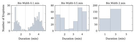
R.The three pictures tell three stories. With bins of 0.1 minutes the histogram is ragged, with empty bins between occupied ones, and the eye is drawn to accidents, such as the single bar of 28 eruptions between 1.8 and 1.9 minutes. With bins of 2 minutes the data collapse into three bars, 97 eruptions under 3 minutes, 171 between 3 and 5, and 4 above, and the picture looks like a single hump with a longer left side. The bins of 0.5 minutes show what the geyser does. Its eruptions come in two kinds, short ones of about 2 minutes and long ones of about 4.3 minutes, and durations near 3 minutes are rare. There is no formula that picks the right bin width; the rule of practice is to try several and to keep the one that shows structure without showing noise, and a reader of a published histogram should ask whether another width would have told a different story.
A histogram is read for its shape, and four words describe most shapes. A distribution is symmetric when its left and right halves are roughly mirror images, as the heights of the men in Figure 3, later in this unit, are. It is skewed to the right when a long tail stretches towards large values, as incomes do (a few people earn very much more than most), and skewed to the left when the tail points towards small values, as the ages at death in a rich country do (most people die old, a few die young). A distribution with one clear peak is unimodal, and one with two peaks, such as the Old Faithful durations, is bimodal; the peak itself is called a mode. Finally, a value that lies far from the bulk of the data is an outlier, and Section 4 gives a precise rule for when a value counts as one. A bimodal histogram usually says that two different groups have been mixed together, and the right response is to find out what separates them. For Old Faithful, a long eruption empties the underground reservoir and is followed by a long wait, so the two kinds of eruption also differ in what follows them.