

Correlation, Regression, and Causation
The closing unit of the Foundation masterclass measures the relation between two variables with the correlation coefficient, summarizes it with the least-squares line, and asks what such a relation can and cannot show. Galton's family heights give the coefficient, the line, and regression to the mean; Anscombe's quartet shows what one number hides; the kidney stone data reverse a comparison; and the smoking debate, Snow's water companies, and the draft lottery of 1969 show why a randomized experiment settles causation and what an accident of history can borrow from one.
Almost every number in the news that is worth arguing about is a claim about two variables at once: that children of tall parents are tall, that richer countries live longer, that smokers die of lung cancer, that a new school raises test scores. The first seven units described one variable at a time and compared it between groups. This unit, the last of the Foundation masterclass, teaches how the relation between two quantitative variables is measured with the correlation coefficient, how it is summarized by a straight line, and why such a relation, however strong, says nothing by itself about cause and effect. It ends with the one design that does settle causation, the randomized experiment, and with the accidents of history that sometimes stand in for one.
1 Scatter plots and the correlation coefficient
Two quantitative variables measured on the same cases, such as the height of a person’s parents and the person’s own height, are plotted as a scatter plot: one dot per case, one variable on each axis. Figure 1 shows the oldest famous scatter plot in statistics, drawn from the family records that Francis Galton (1822-1911) collected in the 1880s. Each of the 934 dots is one adult child. The horizontal position is the mid-parent height, Galton’s name for the average of the father’s height and 1.08 times the mother’s height, with the factor 1.08 chosen because women are on average about 8 per cent shorter than men, so that a mother’s height is put on the scale of a father’s; the vertical position is the child’s own height. Galton measured in inches, and the figure converts to centimetres.
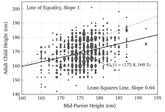
HistData::GaltonFamilies.A scatter plot is read for four things, in this order. The direction of the relation is positive when large values of one variable go with large values of the other, as in Figure 1, and negative when large values of one go with small values of the other, as for the age of a used car and its price. The form is the shape of the cloud: a straight band, a curve, or no pattern at all. Figure 4, later in this unit, shows the same data as a straight band in its right panel and as a curve in its left panel, which is a warning that the form depends on how the axes are drawn. The strength is how tightly the dots follow the form, and the rest of this section turns it into a number. Finally, the plot is searched for outliers, dots that lie far from the pattern of the others, because a single one can change every number computed from the data.
1.1 Covariance and correlation
Unit 2 introduced the \(z\)-score, \(z = (x - \bar{x})/s\), which says how many standard deviations a value lies above or below the mean of its own variable. The \(z\)-score is the natural tool for a relation between two variables measured on different scales, because it removes the scales. If a child whose parents are above average in height is itself above average, the two \(z\)-scores of that child have the same sign and their product is positive; if the parents are tall and the child is short, the product is negative. Averaging these products over all cases gives one number that is positive for a positive relation, negative for a negative one, and near zero when the signs fall at random.
If the products are averaged without first dividing by the standard deviations, the result carries the units of the two variables. The covariance of \(x\) and \(y\) is \[ s_{xy} = \frac{1}{n - 1}\sum_{i=1}^{n}(x_i - \bar{x})(y_i - \bar{y}) , \] with the same \(n - 1\) as the sample variance of Unit 2, and it is measured in the product of the two units of measurement, centimetres times centimetres in Galton’s data. Its size therefore depends on the units of measurement chosen, and that is why the standardized version is the one everybody uses.