

Probability and Conditional Probability
Probability is the language in which every later unit states how sure it is. This unit teaches what a probability means and the three axioms it obeys, how to count outcomes with factorials and binomial coefficients, how information changes a probability, and how Bayes' theorem turns the accuracy of a medical test into the chance that a positive result is right. The birthday problem, the Monty Hall problem, the lady tasting tea, and the case of Sally Clark show the rules at work and the cost of breaking them.
Every claim in the later units of this program, from the margin of error of a poll to the p-value of a clinical trial, is a statement about chance, and chance has rules. The rules are few, they were written down in their final form less than a century ago, and they are easy to misuse. This unit teaches what a probability is, how probabilities are added, multiplied, and counted, and how a probability changes when new information arrives. The last of these ideas, conditional probability, is the tool that lets a reader say what a positive test result means, and the unit ends with a court case in which it was misread.
1 What probability means
Toss a coin a few times and the proportion of heads jumps around. Toss it a few thousand times and the proportion settles down near one half and stays there. In the view that the Foundation units of this program work with, the probability of an event is the proportion of times the event occurs in a very long series of repetitions under the same conditions. To say that the probability of heads is one half is to say that in the long run about half of the tosses land heads, and nothing more. This is called the frequency interpretation of probability, and it fits anything that can be repeated, such as tosses, throws, draws, births, and claims on an insurance policy.
There is a second way to use the word. A historian who says that a manuscript is probably by a certain author is not describing a long run of repetitions, because there is only one manuscript. The number expresses a degree of belief in a statement, on a scale from 0 (certainly false) to 1 (certainly true). Both uses obey the same rules, which is why one unit can serve both, and the degree-of-belief view returns later in the program as a method of inference. Until then, a probability is a long-run proportion.
1.1 Sample spaces and events
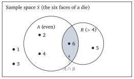
The language of probability starts with a random experiment, which is any action whose result is not known in advance: one throw of a die, one draw of a card, the birth of a child. The sample space \(S\) is the set of all possible outcomes of the experiment. For one throw of a die it is \(S = \{1, 2, 3, 4, 5, 6\}\). An event is a set of outcomes, that is, a statement about the result that is either true or false once the experiment is done. For example, the event \(A\) that the die shows an even number is the set \(\{2, 4, 6\}\), and the event \(B\) that it shows more than 4 is \(\{5, 6\}\).
Events are combined like sets, and three combinations are needed throughout the unit:
- \(A \cap B\) (read “\(A\) and \(B\)”) is the event that both occur. For the die it is \(\{6\}\).
- \(A \cup B\) (read “\(A\) or \(B\)”) is the event that at least one of the two occurs. For the die it is \(\{2, 4, 5, 6\}\). In probability “or” always includes the case that both happen.
- \(A^{c}\) (read “not \(A\)”, the complement of \(A\)) is the event that \(A\) does not occur. For the die it is \(\{1, 3, 5\}\).
Two events that cannot both occur, such as “even” and “odd”, are called mutually exclusive; their intersection is empty. Figure 1 draws the die example as areas, which is how the rules below are easiest to see.
1.2 The axioms
In 1933 Andrey Kolmogorov (1903-1987) published a short book, Grundbegriffe der Wahrscheinlichkeitsrechnung, which put probability on the same footing as the rest of mathematics by stating three rules from which everything else follows. They are known as Kolmogorov’s axioms.