Image: Galton boards of the Matemateca collection, IME-USP; exhibit by Estes Objethos Atelier, photograph by Rodrigo Tetsuo Argenton, CC BY-SA 4.0
A poll of 1,000 people speaks for a country, and 2.4 million ballots once named the wrong president. This unit explains how a random sample is drawn, why bias does not shrink with size, and how far the mean of a sample can stray from the mean of its population. It draws thousands of samples from real data, derives the standard error, states the law of large numbers and the central limit theorem with their conditions, and ends with the Galton board and the margin of error of a poll.
Sample unit: the complete text
An opinion poll of 1,000 people is reported with a margin of error of about 3 percentage points, whether the country has five million voters or two hundred million. A national health survey measures about 5,000 people a year and speaks for a whole country. In 1936 a magazine collected 2.4 million ballots and named the wrong winner. This unit explains how a sample is drawn so that it can stand for a population, what goes wrong when it is not, and the two theorems that say how far the mean of a sample can stray from the mean of the population it came from. It uses the mean and the standard deviation of a set of numbers and the idea of a probability distribution, each recalled in one sentence where it is needed, so that it can be read on its own.
1 Populations and samples
The population is the entire set of cases about which a statement is to be made, and the sample is the part of it that is actually observed. A number that describes the population, such as the mean height of all adult men in a country, is a parameter; the corresponding number computed from the sample, such as the mean height of the 2,500 men whom a health survey actually measured, is a statistic. Parameters are fixed and usually unknown, statistics are known and vary from sample to sample, and this unit is about the relation between the two.
Between the population and the sample stands a list, the sampling frame, which is the list of cases from which the sample is actually drawn, such as an electoral register, a file of postal addresses, a directory of telephone numbers, or the enrolment list of a school. In the best case the frame and the population are the same. Often they are not, and then the sample can only represent the frame. A survey drawn from landline telephone numbers says nothing about households without a landline, however carefully the numbers are drawn, and this gap between the frame and the population is the first place where a survey can go wrong.
1.1 The simple random sample
A simple random sample of size \(n\) is drawn in such a way that every possible set of \(n\) cases in the frame has the same chance of being the set chosen. Two consequences follow at once: each case has the same chance \(n/N\) of being selected, where \(N\) is the number of cases in the frame, and no case is more likely than another to appear together with a given one, which means that whether one case is chosen has no effect on which other cases are chosen with it. The second property is the one that matters, because it is what rules out any connection between who is chosen and what is measured, and the formulas of this unit assume it.
In practice the cases in the frame are numbered from 1 to \(N\), a sequence of random numbers between 1 and \(N\) is produced, and the cases whose numbers come up are the sample, with repeats skipped. The random numbers are the difficult part, because people are bad at inventing them: asked to write down random digits, they avoid repeats and runs of the same digit, which true random digits contain. In 1927 L. H. C. Tippett (1902-1985) published the first table of random digits, 41,600 of them, taken from the figures of a census report, and for decades statisticians drew their samples by reading such tables. Today a computer produces the numbers with a pseudo-random generator, a formula that turns a starting number, the seed, into a long sequence that passes the standard statistical tests of randomness. The same seed gives the same sequence, which is a virtue rather than a flaw: anyone who knows the seed can repeat the draw exactly, and every simulation in this unit states its seed for that reason.
To illustrate this, the health survey behind many of the examples below measured 2,500 men aged 20 and over in one two-year cycle. To draw a simple random sample of 25 of them, number the men from 1 to 2,500, read four-digit groups from a table or a generator, keep each group between 0001 and 2500 that has not come up before, and stop at the twenty-fifth. Nothing about the men so chosen, their height, their age, or their address, played any part in their selection.
1.2 Other ways of drawing a sample
A simple random sample is the design against which all others are measured, and three others are used because they are cheaper, more precise, or more practical.
A stratified sample divides the frame into groups called strata, such as regions or age bands, and draws a simple random sample within each. Every stratum is then represented in known proportion, and a small group of special interest can be sampled more heavily than its share of the population, which is called oversampling; afterwards each stratum’s result is given the weight of the stratum’s true share of the population, so that the oversampled group does not distort the total.
A cluster sample draws groups rather than individuals, for example schools rather than pupils or city blocks rather than households, and then observes every case in the chosen groups or a random sample of them. It saves travel and time, and it costs precision, because people in one cluster tend to resemble each other, so that a cluster of 30 neighbours tells us less than 30 people scattered across the country.
A systematic sample takes every \(k\)-th case from the list after a random start. It is easy to carry out on a production line or a filing cabinet, and it is as good as a simple random sample unless the list has a cycle of length \(k\). For example, if the list is a list of days and \(k = 7\), every chosen day is the same day of the week.
Real surveys combine these. The National Health and Nutrition Examination Survey (NHANES) of the United States, whose height data appear throughout this unit, examines about 5,000 people a year in mobile examination centres. It first draws counties, then neighbourhoods within the counties, then households, then persons, and it deliberately oversamples some groups, among them Hispanic, non-Hispanic Black, and non-Hispanic Asian persons, people on low incomes, and people aged 80 and over, so that it can report on each of them with enough precision. The formulas of this unit are those of a simple random sample. The published results of such a survey are weighted for its design, which goes beyond the unit, so the heights below are used unweighted, as a population to draw from.
2 Bias and variability
A statistic can miss its parameter for two different reasons, and the whole art of sampling lies in keeping them apart. Bias is a systematic error of the method: the statistic is on average too high or too low, in the same direction sample after sample, because of the way the sample was drawn or the measurements were taken. Variability is the scatter of the statistic from one sample to the next around its own average, which exists because different samples contain different cases. Think of the two as shots at a target whose centre is the parameter: variability is the spread of the shots, and bias is the distance of their centre from the bull’s eye. A large sample makes the shots cluster more tightly, but it does not move the cluster. Variability shrinks as the sample grows; bias does not shrink at all.
Four kinds of bias account for most of the surveys that have gone wrong.
Selection bias arises when the frame or the procedure favours some cases over others: telephone subscribers in the poll of 1936 described below, people who happen to walk past an interviewer outside a gym, patients of one hospital standing in for all patients.
Voluntary response bias arises when people choose themselves into the sample, as in a poll on a website, a questionnaire left on a counter, or a radio show that invites listeners to call in. Those who feel strongly, and those who are angry, answer far more often than the rest.
Non-response bias arises when cases that were properly selected cannot be reached or decline to take part, and those who do answer differ from those who do not. Response rates below 10 per cent are now usual for telephone surveys, which leaves plenty of room for this bias.
Measurement bias arises from the instrument or the question: a scale that reads one kilogram too high, a question that suggests its own answer, a request to state one’s own weight, which most people understate.
The first three concern who ends up in the sample, and the fourth concerns what is recorded about them. None of the four is cured by size, and the most famous failure in the history of polling is the standard illustration of the first three.
Source
Number of People
Roosevelt (%)
Literary Digest returns
2,266,566
42.9
Gallup’s quota sample
about 50,000
55.7
Election result
44.4 million votes
62.5
Table 1. The two polls of 1936 against the result, with Roosevelt’s share of the votes for the two main candidates; the Digest’s figure counts the returned ballots that named one of the two. The Digest was 19.6 percentage points off; Gallup’s 50,000 were 6.8 points off. Data: Literary Digest, 31 October 1936; Gallup’s final pre-election poll; official returns of the 1936 election.
The Literary Digest is not a story about the 1930s. Every online poll, every survey answered by whoever clicks, and every large administrative dataset that records some people and not others faces the same arithmetic, and the research spotlight shows what it looks like with the data of 2016.
3 Sampling distributions and the standard error
Suppose now that the sample is a proper simple random sample, so that bias is out of the way, and only variability remains. How large is it? The question can be answered exactly, and the answer is the most useful single formula of the Foundation units.
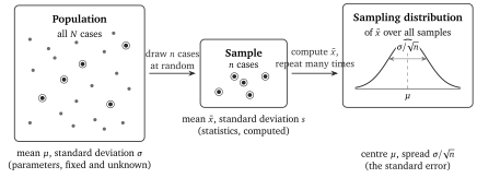
Before the sample is drawn, its mean is unknown; a different set of 25 men would have given a different mean. The sample mean is therefore a random variable, a quantity whose value is decided by chance, and like every random variable it has a probability distribution, the list of the values it can take together with the probabilities of taking them. The distribution of a statistic over all the samples of size \(n\) that could be drawn from the population is called its sampling distribution, and Figure 1 shows the three objects of this unit side by side: the population with its parameters, one sample with its statistics, and the sampling distribution that describes how the statistic varies from sample to sample.
Nobody can draw all possible samples, but a computer can draw a great many, and the worked example does exactly that. Two numbers from the data are needed for it. The mean of a set of values is their sum divided by their number, written \(\mu\) for a population and \(\bar{x}\) for a sample. The standard deviation, written \(\sigma\) for a population and \(s\) for a sample, measures how far the single values typically lie from their mean; it is the square root of the average squared distance from the mean, and for the heights below it is about 7.7 cm, so that a man 7.7 cm above or below the average is a typical rather than an unusual man.
Figure 1. Population, sample, and sampling distribution. A simple random sample of \(n\) cases (ringed dots) is drawn from the population, its mean \(\bar{x}\) is computed, and the process is imagined repeated over and over. The distribution of all those means is the sampling distribution of \(\bar{x}\); it is centred on the population mean \(\mu\) and has the standard deviation \(\sigma/\sqrt{n}\), which is called the standard error.
Sample Size \(n\)
Mean of the 1,000 Means (cm)
SD of the 1,000 Means (cm)
\(\sigma/\sqrt{n}\) (cm)
4
173.54
3.98
3.87
25
173.31
1.57
1.55
100
173.44
0.79
0.77
Table 2. One thousand simulated samples of each size from the 2,500 NHANES men (\(\mu = 173.42\) cm, \(\sigma = 7.74\) cm), drawn with replacement with the seeds 2030, 2051, and 2126. The standard deviation of the sample means follows \(\sigma/\sqrt{n}\) to within the chance variation of the simulation itself.
The formula has two parts. The first, \(\mathrm{E}[\bar{X}] = \mu\), in which \(\mathrm{E}\) stands for the expected value, the average of the sample mean over all the samples that could be drawn, says that the sample mean is right on average, with no systematic tendency to be high or low; a statistic with this property is called unbiased, and it is the mathematical form of the promise that a random sample makes and a self-selected one does not. The second says how far a single sample mean typically lands from \(\mu\), and the square root in its denominator is the most consequential square root in statistics. Capital \(\bar{X}\) denotes the sample mean as a random variable, before the sample is drawn; lower case \(\bar{x}\) is its value in one particular sample.
3.1 The square root law
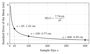
The standard error falls with the square root of the sample size, and the consequence is uncomfortable for anyone who pays for data. Figure 2 draws \(\mathrm{SE}(\bar{x}) = 7.74\unit{cm}/\sqrt{n}\) for the heights. Going from 25 to 100 men, four times the work, halves the standard error from 1.55 to 0.77 cm, and halving it again requires 400 men.
Figure 2. The standard error of the mean height against the sample size, computed from \(\sigma/\sqrt{n}\) with \(\sigma = 7.74\) cm. Each fourfold increase in \(n\) halves the standard error: 1.55 cm at \(n = 25\), 0.77 cm at 100, and 0.39 cm at 400. Data: standard deviation of the heights of 2,500 men aged 20 and over, NHANES 2017 to 2018.
4 The law of large numbers
The standard error shrinks towards zero as \(n\) grows, and this is the quantitative form of an old and famous statement. Jacob Bernoulli (1655-1705) proved in his book Ars Conjectandi, published in 1713 after his death, that the proportion of successes in a long series of independent trials comes as close as one likes to the probability of success, and that it does so with a probability as near to certainty as one likes, provided the series is long enough. He called it his golden theorem; it is now called the law of large numbers, and it holds for means as well as for proportions.
When the population also has a finite standard deviation \(\sigma\), the law follows from the standard error in a few lines through an inequality of Pafnuty Chebyshev (1821-1894), which says that the probability of a deviation of more than \(\varepsilon\) between \(\bar{X}_n\) and \(\mu\) is at most \(\sigma^2/(n\varepsilon^2)\), a bound that goes to zero as \(n\) grows whatever \(\varepsilon\) is. The bound is crude, because it must hold for every shape of population; the next section gives a far sharper statement for large \(n\).
4.1 What the law promises, and what it does not
The law of large numbers is why casinos and insurance companies exist. On a European roulette wheel with 37 pockets, a player who bets one euro on red wins one euro with probability \(18/37\) and loses it with probability \(19/37\), so the expected result is \(-1/37\) of a euro, a loss of 2.7 cents per euro bet. A single player on a single evening may win a great deal, but over the millions of bets a casino takes in a year its average take per euro will be close to 2.7 cents, and its income is as predictable as a factory’s. An insurer who covers 100,000 houses against fire cannot say which of them will burn, but can say almost exactly how many.
What the law does not promise is a correction of the past. Suppose 1,000 tosses of a fair coin have produced 530 heads. The law says that the proportion of heads over the whole series will approach one half as the tossing continues. It does not say that tails are now due. The next 9,000 tosses are expected to split evenly, about 4,500 each, so the expected count after 10,000 tosses is \(5{,}030\) heads against \(4{,}970\) tails: the surplus of 30 heads is expected to persist, and the proportion nevertheless moves from 53.0 per cent to 50.3 per cent, because the same 30 are now divided by 10,000 instead of 1,000. The law works by burying the early surplus under many later tosses, never by compensating for it. The belief that a run of one outcome makes the other more likely is the gambler’s fallacy, and the “law of averages” that is supposed to justify it does not exist.
5 The central limit theorem
The law of large numbers says where the sample mean goes; the standard error says how far from \(\mu\) it typically is. One more thing can be said, and it is the reason the normal curve appears on almost every page of statistics: the shape of the sampling distribution of the mean is known as well, and it is nearly the same whatever the shape of the population.
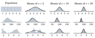
Figure 3. Three populations and the distributions of their sample means. Top row: the six faces of a fair die (uniform). Middle row: the body weights of 5,185 adults aged 20 and over, NHANES 2017 to 2018 (right-skewed; 20 adults heavier than 170 kg lie beyond the right edge). Bottom row: the durations of 272 eruptions of Old Faithful, Azzalini and Bowman (1990), from Rdatasets (bimodal). Each sampling distribution holds the means of 2,000 simulated samples drawn with replacement (seeds 5002 to 5004 for the die, 5010 to 5012 for the weights, and 5030 to 5032 for the geyser, one per sample size); bin widths are 1, 0.5, 0.2, and 0.1 for the die, 5, 5, 2, and 1 kg for the weights, and 0.2, 0.2, 0.1, and 0.05 minutes for the geyser. The curves are the normal density with mean \(\mu\) and standard deviation \(\sigma/\sqrt{n}\) of each population; the vertical scales differ between panels.
Figure 3 shows this for three populations that could hardly be more different. The first is the six faces of a fair die, each equally likely, a flat distribution. The second is the body weight of 5,185 adults measured in NHANES in 2017 and 2018, which is skewed to the right, with a long tail of heavy people. The third is the duration of 272 eruptions of the Old Faithful geyser in Yellowstone National Park, which has two separate humps, short eruptions of about two minutes and long ones of about four and a half. From each population 2,000 samples of size 2, 10, and 30 were drawn with a seeded generator, and the means of the samples were collected into histograms.
Three things happen in every row, and they are the three statements of this unit. The histograms of the means stay centred on the population mean. They become narrower as \(n\) grows, by the factor \(\sqrt{n}\). And they take on the shape of the normal curve drawn over them, whatever the shape they started from: the flat die is almost normal at \(n = 10\), the skewed weights still lean to the right at \(n = 10\) and are very nearly symmetric at \(n = 30\), and the two humps of the geyser, still visible as a ragged shape at \(n = 2\), have merged into a single bell by \(n = 10\). This is the content of the central limit theorem.
The last sentence of the box is where a careful reader should pause. Textbooks often give \(n \ge 30\) as the point from which the normal approximation may be used, and Figure 3 shows why the number is only a habit. For a symmetric population such as the die, or the heights of Section 3, samples of 5 or 10 are already enough. For a moderately skewed population such as the weights, 30 is about right. For a strongly skewed population, such as personal incomes or insurance claims, where a few enormous values dominate the mean, several hundred observations may be needed, and for populations whose tail is so heavy that the variance is not finite at all, and such populations do exist, the theorem makes no promise. The theorem also says nothing about the single observations. A large sample of incomes is just as skewed as a small one; it is the mean of the sample whose distribution becomes normal, and confusing the two is one of the most common misreadings in the subject.
The normal shape is what lets the standard error be read as a probability. A standard normal variable lies within one standard deviation of its centre with probability 68 per cent and within two with probability 95 per cent, so a sample mean lies within one standard error of \(\mu\) in about 68 per cent of samples and within two in about 95 per cent, which is what the simulation of Section 3 found with 674 and 945 of its 1,000 means. The following Key Formula is the bridge to the next units, which turn it into confidence intervals and tests.
5.1 The Galton board
The oldest demonstration of the theorem is a wooden board with rows of pins, and it is also the clearest, because the mechanism that produces the bell shape can be watched one ball at a time. A ball dropped onto the top pin bounces left or right, falls onto the next row, bounces again, and after passing every row drops into one of a row of slots at the bottom. Each bounce is a coin toss, and the slot the ball lands in is decided by how many of its bounces went to the right. Poured through by the hundred, the balls pile up in the slots in a bell shape, as the photograph at the head of this unit shows.
Figure 4. Galton’s drawings of the apparatus in Natural Inheritance (1889). In Fig. 7 the shot poured through the funnel passes the rows of pins and settles in the compartments in a bell-shaped heap. Fig. 8 is the two-stage version: the shot is caught halfway down at A, where it already forms a bell, and each compartment is then released separately through a second bank of pins into the compartments at B. Fig. 9 slopes the lower compartments so that the heaps can be compared. Credit: Francis Galton, Natural Inheritance, Macmillan, 1889, page 63; Internet Archive scan, public domain.
The theorem has a long history. De Moivre’s result of 1733 covered only coin tosses; Pierre-Simon Laplace (1749-1827) extended it in 1810 to sums of arbitrary independent quantities; the Russian mathematician Aleksandr Lyapunov (1857-1918) gave the first rigorous proof of a general version in 1901; and the name, zentraler Grenzwertsatz, was coined by George Pólya (1887-1985) in the title of a paper of 1920, because of the central place the theorem holds in probability. Versions for draws that are not identically distributed exist and go beyond this unit; they are the reason the bell curve appears in measurement errors and in the heights of people, none of which is a coin toss.
6 Proportions and the size of a sample
Everything said about the mean applies to a proportion, because a proportion is a mean in disguise. Give every case the value 1 if it has the property in question and 0 if it does not; then the sum of the values is the count of cases with the property, and their mean is the proportion. In the population the mean of these 0 and 1 values is the proportion \(p\) of cases with the property, and their variance is \(p(1 - p)\), because a value of 1 lies \(1 - p\) above the mean and a value of 0 lies \(p\) below it, and the average of the squared distances, \(p(1 - p)^2 + (1 - p)p^2\), comes to \(p(1 - p)\); it is \(1/4\) at \(p = 1/2\) and smaller elsewhere. The sample proportion \(\hat{p}\), read “p hat”, is the sample mean of the same values, and the Key Formula of Section 3 gives its standard error at once.
6.1 The poll of 1,000 people
The number in the first sentence of this unit now has a source. An opinion poll that interviews a simple random sample of \(n = 1{,}000\) people, in which a candidate’s true share is near one half, measures that share with a standard error of \(\sqrt{0.25/1{,}000} = 0.0158\). Two standard errors, more exactly \(1.96\) of them, come to \(0.031\), and that is the figure of “about 3 percentage points” printed under every such poll; Unit 6 explains exactly what it means and how it becomes a confidence interval. Four times as many interviews, 4,000, bring it to 1.5 points, and 16,000 interviews bring it to 0.8 points. The margin also assumes a simple random sample and a complete response, which no real poll has, and the published margins of serious pollsters are corrected for their actual designs by methods beyond the unit.
One thing is absent from the formula, and its absence surprises most people: the size of the population. The standard error of a sample of 1,000 is the same whether the 1,000 were drawn from a town of 100,000 or from a country of 60 million. The exact formula for a sample drawn without replacement from a finite population of \(N\) cases multiplies \(\sigma/\sqrt{n}\) by the factor \(\sqrt{(N - n)/(N - 1)}\), the finite population correction, which is \(0.995\) for 1,000 out of 100,000 and \(0.99999\) for 1,000 out of 60 million. Only when the sample is a large fraction of the population, more than 5 or 10 per cent of it, does the correction matter, and then it helps. A spoonful of soup tells the cook whether the pot is salted, however large the pot, provided the pot was stirred. The stirring is the random draw, and the Literary Digest’s 2.4 million unstirred spoonfuls are the lesson that no quantity of data makes up for its absence.
This is one of 16 units
Participants also get the quiz, the further reading, and the final exam.