

Logistic Regression and Generalized Linear Models
Many responses are a yes or a no, or a count, and a straight line cannot model them. This unit models the log odds of an event as a straight line, reads the coefficients as odds ratios, and fits the model by maximum likelihood with the Challenger O-ring data as the running example. It turns fitted probabilities into decisions with sensitivity, specificity, and the ROC curve, models counts with a Poisson regression and an offset for exposure, and ends with the generalized linear model that holds linear, logistic, and Poisson regression together, compared by the deviance.
The regressions of Units 8 and 10 predict a quantity measured in centimetres, dollars, or litres. Many of the questions statistics is asked have an answer of a different kind: a patient has diabetes or has not, an O-ring on a rocket booster fails or holds, a loan is repaid or not, and a football team scores 0, 1, 2, or more goals. This unit extends regression to such responses. It introduces odds and the logistic curve, fits the model by the maximum likelihood method of Unit 9, turns the fitted probabilities into decisions and measures how good those decisions are, extends the same idea to counts, and ends with the framework that holds the linear, the logistic, and the Poisson regression together as one family.
1 Binary responses and odds
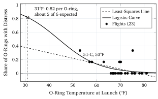
A binary response is a variable \(Y\) that takes only the values 1 (the event happens) and 0 (it does not). Its mean is the probability of the event, \(\mathrm{E}[Y] = \mathrm{P}(Y = 1) = p\), so a regression of a binary response is a model for a probability. The first idea is to use the straight line of Unit 8, \(p = \beta_0 + \beta_1 x\), and Figure 1 shows why statisticians abandoned it.
The figure plots the data that run through this unit. Before the flight of the Space Shuttle Challenger on 28 January 1986, the shuttle had flown 24 times, and for 23 of those flights the two solid rocket boosters had been recovered from the sea and inspected (the boosters of one flight were lost). Each booster has three field joints sealed by O-rings of rubber, six primary O-rings per flight, and the inspections recorded how many of the six showed thermal distress, that is, erosion by hot gas or gas blowing past the ring. The horizontal axis is the temperature of the O-rings at launch, which the engineers calculated for each flight from the air temperature of the preceding hours, and it runs from 53 to 81 °F (about 12 to 27 °C). The vertical axis is the share of the six O-rings with distress. That share is 0 for 16 flights, 1 in 6 for five flights, and 2 in 6 for two flights, which makes 9 distressed O-rings among the 138 inspected. The dashed line is the least-squares line fitted to these shares. It predicts a negative share for every launch warmer than 78 °F, which is nonsense for a probability, and it predicts a share of 0.37 at 31 °F, a figure that depends on the line continuing straight far outside the data. A straight line has two further faults for a probability. The variance of a binary variable is \(p(1 - p)\), as Unit 4 found for a Bernoulli trial, and it changes with \(x\) because \(p\) does, so the constant-variance condition of the Gauss-Markov theorem of Unit 10 fails. And a line says that each degree changes the probability by the same amount at every temperature, whereas a probability near 0 or 1 has no room left to change.
The remedy is to model a transformed probability that has no upper or lower limit. The odds of an event are the probability that it happens divided by the probability that it does not: \begin{equation} \text{odds} = \frac{p}{1 - p} . \label{eq:odds} \end{equation} A probability of 0.75 is odds of \(0.75/0.25 = 3\), or three to one; a probability of one half is odds of 1, or one to one; a probability of 0.1 is odds of \(1/9\). Odds run from 0 to infinity, and the logarithm of the odds, called the log odds or the logit, runs from minus infinity to plus infinity, with 0 at a probability of one half, \(+1.10\) at \(0.75\), and \(-1.10\) at \(0.25\). The logit is also symmetric, in the sense that the log odds of an event and of its opposite differ only in sign, since \(\ln\bigl((1 - p)/p\bigr) = -\ln\bigl(p/(1 - p)\bigr)\). A straight line on the logit scale can therefore run on forever in both directions and still correspond to a probability between 0 and 1.