

Bayesian Inference
Bayes' theorem turns a prior distribution and a likelihood into a posterior distribution for a parameter, and the unit works this through in full for a proportion, where a Beta prior and binomial data give a Beta posterior, and for a mean, where precisions add. It explains what a credible interval promises and what a confidence interval promises, how to choose a prior and show that it did not decide the result, why a batting average after 30 at-bats is shrunk towards the league, and how the Metropolis algorithm draws samples from a posterior that nobody can write down, with the diagnostics that say whether the run can be trusted.
Unit 9 read the probability of the data backwards, as a function of the unknown parameter, and called the result the likelihood. It was careful to say that a likelihood is not a probability distribution for the parameter, and this unit supplies the missing ingredient. If the parameter is given a probability distribution before the data are seen, Bayes’ theorem of Unit 3 turns the likelihood into a probability distribution for the parameter after the data are seen, and the questions a researcher actually asks (how probable is it that the coin favours heads, that the new treatment helps, that the batter is better than average) get direct answers. The price is the distribution before the data, called the prior, and much of the unit is about paying that price honestly. The last section shows how a computer draws samples from a distribution that nobody can write down, which is why a method born in 1763 became practical only in the 1990s.
1 Bayes’ theorem for a parameter
Unit 3 stated Bayes’ theorem for two events, \(\mathrm{P}(A \mid B) = \mathrm{P}(B \mid A)\,\mathrm{P}(A)/\mathrm{P}(B)\), and used it to turn the sensitivity of a medical test into the probability of disease given a positive result. The same theorem applies to a parameter. Let \(\theta\) be the unknown quantity, such as the probability \(p\) that a coin lands heads, and let \(x\) stand for the data, such as the 51 heads in 100 tosses that Units 4, 6, and 9 have used. Three distributions take part:
- the prior distribution \(f(\theta)\), the probability distribution of \(\theta\) before the data are seen, which collects what is known or assumed about the parameter from outside the data;
- the likelihood \(f(x \mid \theta)\), the probability of the data given the parameter, which is the function \(L(\theta)\) of Unit 9 written with its arguments;
- the posterior distribution \(f(\theta \mid x)\), the probability distribution of \(\theta\) after the data have been taken into account.
Bayes’ theorem links the three, and the key formula states how.
The denominator deserves a sentence, because it frightens beginners and is never computed. The quantity \(f(x)\) is the probability of the data averaged over all values of the parameter, each weighted by its prior probability; it is called the marginal likelihood, and its only role in the theorem is to make the right-hand side a proper density, one with total area one. Because it is the same number for every \(\theta\), one may ignore it while working and divide by the total area at the end, and that is what the symbol \(\propto\) (“is proportional to”) says. The same reasoning let Unit 9 drop the binomial coefficient from the likelihood: a constant factor changes nothing about the shape of the curve, and only the shape carries information. Many Bayesian textbooks write \(p(\theta)\), \(p(x \mid \theta)\), and \(p(\theta \mid x)\) for all three distributions; this program writes \(f\) for a density and keeps \(p\) for a proportion, as it has since Unit 1.
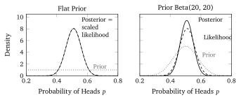
To illustrate the theorem with the coin, take the prior that treats every value of \(p\) between 0 and 1 as equally plausible, \(f(p) = 1\), called the flat prior or uniform prior. The likelihood of 51 heads in 100 tosses is proportional to \(p^{51}(1 - p)^{49}\), as in Unit 9. The posterior is therefore \[ f(p \mid \text{51 heads in 100}) \propto p^{51}(1 - p)^{49} \times 1 , \] and the whole content of the data, as a probability statement about \(p\), is the curve on the left of Figure 1: a density that peaks at \(0.51\) and is almost zero below \(0.35\) and above \(0.67\). With a flat prior the posterior is the likelihood curve scaled to have area one, and nothing else. The right panel shows what a prior does. A reader who believed before the tosses that the coin is close to fair, and expressed this by a prior concentrated around one half, ends with a posterior that lies between the prior and the likelihood and is narrower than either, because two sources of information have been combined. Section 2 gives the formulas behind both panels.