

Likelihood and Maximum Likelihood
The first unit of the Advanced masterclass shows where the estimates of the Foundation units come from. The probability formula of a model is read backwards, as a function of the unknown parameter with the data held fixed, and the value that makes the observed data most probable is the maximum likelihood estimate. The unit teaches the derivative before it uses it, derives the estimates of a proportion, a Poisson rate, and a normal mean and variance, reads the standard error from the curvature of the log-likelihood, and turns the drop in log-likelihood into a test and an interval, with coin flips, horse kicks, geysers, earthquakes, and the words of Moby-Dick as the data.
Unit 4 gave the formula for the probability of any number of heads in 100 tosses of a coin that lands heads with probability \(p\), and Units 5 to 8 estimated proportions, means, and regression slopes with formulas that arrived ready-made: the sample proportion, the sample mean, the least-squares line. This unit shows where such formulas come from. The idea, worked out by Ronald Fisher (1890-1962) between 1912 and 1922, is to read the probability formula backwards, as a function of the unknown parameter with the data held fixed, and to pick the parameter value that makes what was actually observed most probable. The method is called maximum likelihood. It returns the familiar estimates in the familiar cases, it works just as well where no familiar formula exists, and it brings its own standard errors and tests; the regression models of Units 10 and 11 and the Bayesian inference of Unit 12 are built on it. On the way, the unit teaches the one piece of calculus that the Advanced units need, the derivative, in the form in which statisticians use it.
1 From probability to likelihood
Unit 4 stated the binomial formula. If a coin lands heads with probability \(p\) and is tossed \(n\) times independently, the number of heads \(X\) has \begin{equation} \mathrm{P}(X = k) = \binom{n}{k}\,p^{k}(1 - p)^{n - k} , \qquad k = 0, 1, \ldots, n . \label{eq:binom} \end{equation} Unit 4 read this formula forwards. The parameter \(p\) was known, \(k\) varied, and the formula distributed the total probability of one over the possible counts, which is why the probabilities over all \(k\) add up to one. A statistician who has just counted 51 heads in 100 tosses reads the same formula backwards. The count is now fixed at \(k = 51\) and \(n = 100\), and the unknown is \(p\). For every candidate value of \(p\) the formula says how probable the observed count would have been, and this number, read as a function of the parameter, is called the likelihood of \(p\) and written \(L(p)\). For the 100 tosses, \[ L(p) = \binom{100}{51}\,p^{51}(1 - p)^{49} , \qquad 0 < p < 1 . \] The left panel of Figure 1 draws it. The curve is zero at both ends, because a coin that never lands heads cannot produce 51 heads and neither can one that always does, and it has a single hump whose top sits at \(p = 0.51\), the sample proportion. For example, \(L(0.6)/L(0.51) = 0.19\), and since \(1/0.19 = 5.3\) the observed count is about five times as probable under \(p = 0.51\) as under \(p = 0.6\), whereas \(L(0.5)/L(0.51) = 0.98\), so a fair coin explains the data almost as well as the best value does.
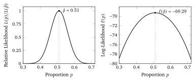
Two things about this function must be said at once, because they are misread more often than anything else in the unit. First, the binomial coefficient \(\binom{100}{51}\) does not depend on \(p\). It multiplies the whole curve by the same number and so cannot move the maximum or change any ratio of two likelihoods, and it is dropped from now on. A likelihood is defined only up to a constant factor, which means that multiplying it by any fixed number gives an equally valid likelihood, and only ratios of likelihoods carry information, which is why Figure 1 plots \(L(p)\) relative to its largest value. Second, \(L(p)\) is not a probability distribution for \(p\). The area under the curve is not one and need not be, and \(L(0.6) = 0.19\) does not mean that there is a 19 per cent chance that \(p\) is \(0.6\). The likelihood answers the question “how probable were these data if the parameter were \(p\)”, and the question “how probable is this value of \(p\) given the data” needs one more ingredient, a probability for \(p\) before the data were seen, which Unit 12 supplies. Fisher chose the word likelihood in 1921 to keep the two questions apart.