

Hypothesis Tests and p-Values
A difference in a sample can be a real effect or the ordinary wobble of chance, and a hypothesis test is the controlled way to tell the two apart. This unit builds the test on Fisher's lady tasting tea, defines the p-value exactly, carries out the z, t, paired, and two-sample tests, sets out the two kinds of error and the power of a test, plans the size of a trial, tests two proportions on Snow's water companies and tables of counts on Mendel's peas and Doll and Hill's smokers, and ends with what a p-value is not.
Ten patients slept on average 1.58 hours longer under one drug than under another, and 5,474 round peas stood against 1,850 wrinkled ones where a theory predicted three to one. Both numbers could be the trace of a real effect, and both could be the ordinary variation of a sample that Units 5 and 6 described. A hypothesis test is the procedure statisticians use to decide between these two readings in a controlled way, with a known rate of mistakes. This unit builds the procedure on a cup of tea, applies it to means, proportions, and tables of counts, and ends with what its number, the p-value, can and cannot say.
1 The logic of a test
1.1 Null hypothesis, test statistic, and p-value
Unit 3 counted the ways of choosing 4 cups out of 8 and found 70. The count was part of an experiment that Ronald Fisher (1890-1962) described in The Design of Experiments (1935), in which a lady claims that she can taste whether the milk or the tea was poured into the cup first. Fisher’s design presents her with 8 cups, 4 of each kind in random order, tells her so, and asks her to name the 4 cups with milk first. The same experiment now serves to define the parts of a test.
The null hypothesis, written \(H_0\), is the statement that nothing is going on, made precise enough to compute with. Here it says that the lady cannot tell the difference, so that her choice of 4 cups is, as far as the outcome is concerned, a random pick out of the 70 possible choices. The alternative hypothesis \(H_1\) is the statement the experiment is looking for, which is that she can tell. The test statistic is the number computed from the data that measures how far the result is from what the null hypothesis leads one to expect, and here it is the number of correctly named cups, which can be 0, 1, 2, 3, or 4. The last ingredient is a rule for turning the observed value of the statistic into a judgement.
The procedure is known as Fisher’s exact test, exact because the probability is computed by counting rather than from an approximating curve. The quantity at its heart deserves its own definition. The p-value is the probability, computed as if the null hypothesis were true, of obtaining a test statistic at least as extreme as the one actually observed: \begin{equation} \text{p-value} = \mathrm{P}(\text{a result at least as extreme as the observed one} \mid H_0 \text{ true}) . \label{eq:pvalue} \end{equation} Every word of this sentence matters, and Section 5 returns to the words that are most often dropped. Two of its parts need attention at once. The condition in Equation \eqref{eq:pvalue} is that \(H_0\) is true; the p-value is a statement about the data given the hypothesis, in the same way that \(\mathrm{P}(B \mid A)\) in Unit 3 is a statement about \(B\) given \(A\), and it is not the probability of the hypothesis given the data. The phrase “at least as extreme” includes the observed result and everything further from \(H_0\), because a single exact value, such as exactly 3 correct cups, is not what makes a result surprising; what makes it surprising is that it lies so far out in the tail.
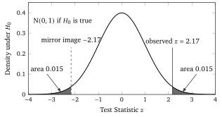
For a test statistic with a continuous distribution the p-value is an area under the null distribution, as in Figure 1. When the alternative hypothesis allows a difference in either direction, both tails count and the test is two-sided; Section 2 says when a one-sided test is justified.